Calculating with Uncertainties: from a Point to a Distribution
Engineering calculations generally use point values as input.
A car with a speed of 100 km/h will go a distance of 1.66 km in one minute. As long as the input variables of the calculation are exactly known and there is a clear relationship between the variables, exactly one value is derived as a result. If, however, the speed is measured, deviations can occur which, for example, are indicated by ± 10%. Thus, one speed turns into two: 90 km/h and 110 km/h. The same applies to the result: 1.50 km and 1.83 km or 1.66 km ± 10%.
If deviations occur with both input variables, the number of possible results expands to four: the true value thus lies between 1.43 km and 1.93 km.

Due to a higher number of input values and more complicated mathematical relationships between the values, the effect of the deviations can no longer be directly predicted, as in the example above. The next step in considering uncertainties is the transition to the use of distributions instead of the extreme values. In the simplest case, a uniform distribution is obtained; the speed could be any value between 90 km/h and 110 km/h, the mean value is again 100 km/h. There are two basic cases:
- Discrete distributions: The range of values is divided into a countable set of equally large sections; Here, for example, 1 km/h, then 21 values are obtained between 90 km/h and 110 km/h (90,91,92,93,94, ...,106,107,108,109,110).
- Continuous (steady) distributions: The magnitude takes on any value in the value range; The magnitude must be represented by a function.

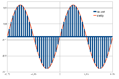
The decisive difference with this extended concept is simply explained by the sine function. Suppose the observed size has a mean of 0 and can be any value between ± 2Π. The function value is zero for the mean value and the two extreme values, but in between it assumes all values between -1 and +1.
While it would theoretically be possible to perform the calculation according to the initial example in the discrete case, the use of continuous distributions requires a different mathematical treatment of the problem. One possibility is the so-called Monte Carlo method. In this case, a value (realization) is selected randomly for each distributed input parameter, and the calculation is performed with it. This process is repeated very often, generating results based on the number of repetitions (games). The result of the calculation can again only be represented as a distribution.
This method is used in the simulation of a regenerative energy supply system that is not connected to the power supply grid, for example. This includes, among other things, the weather (influence on electricity generation with wind and photovoltaics) and the consumption of uncertain amounts, which are represented by a distribution. The result is a statement on the number of investigated cases where the system is unable to meet the consumer's needs.


